Beginning Machine Learning with Keras & Core ML
In this Keras machine learning tutorial, you’ll learn how to train a convolutional neural network model, convert it to Core ML, and integrate it into an iOS app. By Audrey Tam.
Dense
Dense(128, activation='relu')
Dense(num_classes, activation='softmax')
Each neuron in a convolutional layer uses the values of only a few neurons in the previous layer. Each neuron in a fully connected layer uses the values of all the neurons in the previous layer. The Keras name for this type of layer is Dense.
Looking at the model summaries above, Malireddi’s first Dense layer has 512 neurons, while Chollet’s has 9216. Both produce a 128-neuron output layer, but Chollet’s must compute 18 times more parameters than Malireddi’s. This is what uses most of the additional training time.
Most CNN architectures end with one or more Dense layers and then the output layer.
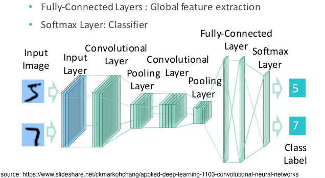
The first parameter is the output size of the layer. The final output layer has an output size of 10, corresponding to the 10 classes of digits.
The softmax activation function produces a probability distribution over the 10 output classes. It’s a generalization of the sigmoid function, which scales its input value into the range [0, 1]. For your MNIST classifier, softmax scales each of 10 values into [0, 1], such that they add up to 1.
You would use the sigmoid function for a single output class: for example, what’s the probability that this is a photo of a good dog?
Compile
model_m.compile(loss='categorical_crossentropy', optimizer='adam', metrics=['accuracy'])
The categorical crossentropy loss function measures the distance between the probability distribution calculated by the CNN, and the true distribution of the labels.
An optimizer is the stochastic gradient descent algorithm that tries to minimize the loss function by following the gradient down at just the right speed.
Accuracy — the fraction of the images that were correctly classified — is the most common metric monitored during training and testing.
Fit
batch_size = 256
epochs = 10
model_m.fit(x_train, y_train, batch_size=batch_size, epochs=epochs, callbacks=callbacks_list,
            validation_data=(x_val, y_val), verbose=1)
Batch size is the number of data items to use for mini-batch stochastic gradient fitting. Choosing a batch size is a matter of trial and error, a roll of the dice. Smaller values make epochs take longer; larger values make better use of GPU parallelism, and reduce data transfer time, but too large might cause you to run out of memory.
The number of epochs is also a roll of the dice. Each epoch should improve loss and accuracy measurements. More epochs should produce a more accurate model, but training takes longer. Too many epochs can result in overfitting. You set up a callback to stop early, if the model stops improving before completing all the epochs. In the notebook, you can re-run the fit cell to keep improving the model.
When you loaded the data, 10000 items were set as validation data. Passing this argument enables validation while training, so you can monitor validation loss and accuracy. If these values are worse than the training loss and accuracy, this indicates that the model is overfitted.
Verbose
0 = silent, 1 = progress bar, 2 = one line per epoch.
Results
Here’s the result of one of my training runs:
Epoch 1/10
60000/60000 [==============================] - 106s - loss: 0.0284 - acc: 0.9909 - val_loss: 0.0216 - val_acc: 0.9940
Epoch 2/10
60000/60000 [==============================] - 100s - loss: 0.0271 - acc: 0.9911 - val_loss: 0.0199 - val_acc: 0.9942
Epoch 3/10
60000/60000 [==============================] - 102s - loss: 0.0260 - acc: 0.9914 - val_loss: 0.0228 - val_acc: 0.9931
Epoch 4/10
60000/60000 [==============================] - 101s - loss: 0.0257 - acc: 0.9913 - val_loss: 0.0211 - val_acc: 0.9935
Epoch 5/10
60000/60000 [==============================] - 101s - loss: 0.0256 - acc: 0.9916 - val_loss: 0.0222 - val_acc: 0.9928
Epoch 6/10
60000/60000 [==============================] - 100s - loss: 0.0263 - acc: 0.9913 - val_loss: 0.0178 - val_acc: 0.9950
Epoch 7/10
60000/60000 [==============================] - 87s - loss: 0.0231 - acc: 0.9920 - val_loss: 0.0212 - val_acc: 0.9932
Epoch 8/10
60000/60000 [==============================] - 76s - loss: 0.0240 - acc: 0.9922 - val_loss: 0.0212 - val_acc: 0.9935
Epoch 9/10
60000/60000 [==============================] - 76s - loss: 0.0261 - acc: 0.9916 - val_loss: 0.0220 - val_acc: 0.9934
Epoch 10/10
60000/60000 [==============================] - 76s - loss: 0.0231 - acc: 0.9925 - val_loss: 0.0203 - val_acc: 0.9935
With each epoch, loss values should decrease, and accuracy values should increase. The ModelCheckpoint callback saves epochs 1, 2 and 6, because validation loss values in epochs 3, 4 and 5 are higher than epoch 2’s, and there’s no improvement in validation loss after epoch 6. Training doesn’t stop early, because training accuracy never decreases for two consecutive epochs.
fit cell more than once, without resetting the model, so loss and accuracy values are already quite good, even in epoch 1. But you see some wavering in the measurements, for example, accuracy decreases in epochs 4, 6 and 9.
By now, your model has finished training, so back to coding!
Convert to Core ML Model
When the training step is complete, you should have a few models saved in notebook. The one with the highest epoch number (and lowest validation loss) is the best model, so use that filename in the convert function.
Enter the following code, and run it.
output_labels = ['0', '1', '2', '3', '4', '5', '6', '7', '8', '9']
# For the first argument, use the filename of the newest .h5 file in the notebook folder.
coreml_mnist = coremltools.converters.keras.convert(
    'best_model.09-0.03.h5', input_names=['image'], output_names=['output'],
    class_labels=output_labels, image_input_names='image')
Here, you set the 10 output labels in an array, and pass this as the class_labels argument. If you train a model with a lot of output classes, put the labels in a text file, one label per line, and set the class_labels argument to the file name.
In the parameter list, you supply input and output names, and set image_input_names='image' so the Core ML model accepts an image as input, instead of a multi-array.
Inspect Core ML model
Enter this line, and run it to see the printout.
print(coreml_mnist)
Just check that the input type is imageType, not multi-array:
input {
  name: "image"
  shortDescription: "Digit image"
  type {
    imageType {
      width: 28
      height: 28
      colorSpace: GRAYSCALE
    }
  }
}