Beginning Machine Learning with Keras & Core ML

Keras Code Time!

OK, the Docker container should be ready now: go back and follow the instructions to open the notebook. It’s time to write some Keras code!

Enter the following code in the keras_mnist.ipynb cell with the matching heading. When you finish entering the code in each cell, press Control-Enter to run it. An asterisk appears in the In [ ]: label while the code is running, then a number will appear, to show the order in which you ran the cells. Everything stays in memory while you’re logged in to the notebook. Every so often, tap the Save and Checkpoint button.

Import Utilities & Dependencies

Enter the following code, and run it to check the Keras version.

from __future__ import print_function
from matplotlib import pyplot as plt

import keras
from keras.datasets import mnist
from keras.models import Sequential
from keras.layers import Dense, Dropout, Flatten
from keras.layers import Conv2D, MaxPooling2D
from keras.utils import np_utils
from keras import backend as K

import coremltools
# coremltools supports Keras version 2.0.6
print('keras version ', keras.__version__)

__future__ is the compatibility layer between Python 2 and Python 3: Python 2 has a print command (no parentheses), but Python 3 requires a print() function. Importing print_function allows you to use print() statements in Python 2 code.

Keras uses the NumPy mathematics library to manipulate arrays and matrices. Matplotlib is a plotting library for NumPy: you’ll use it to inspect a training data item.

After importing keras, print its version: coremltools supports version 2.0.6, and will spew warnings if you use a higher version. Keras already has the MNIST dataset, so you import that. Then the next three lines import the model components. You import the NumPy utilities, and you give the backend a label with import backend as K: you’ll use it to check image_data_format.

Finally, you import coremltools, which you’ll use at the end of this notebook.

Load & Pre-Process Data

Training & Validation Data Sets

First, get your data! Enter the code below, and run it: downloading the data takes a little while.

(x_train, y_train), (x_val, y_val) = mnist.load_data()

This downloads data from https://s3.amazonaws.com/img-datasets/mnist.npz, shuffles the data items, and splits them between a training dataset and a validation dataset. Validation data helps to detect the problem of overfitting the model to the training data. The training step uses the trained parameters to compute outputs for the validation data. You’ll set callbacks to monitor validation loss and accuracy, to save the model that performs best on the validation data, and possibly stop early, if validation loss or accuracy fail to improve for too many epochs (repetitions).

Inspect x & y Data

When the download finishes, enter the following code in the next cell, and run it to see what you got.

# Inspect x data
print('x_train shape: ', x_train.shape)
# Displays (60000, 28, 28)
print(x_train.shape[0], 'training samples')
# Displays 60000 train samples
print('x_val shape: ', x_val.shape)
# Displays (10000, 28, 28)
print(x_val.shape[0], 'validation samples')
# Displays 10000 validation samples

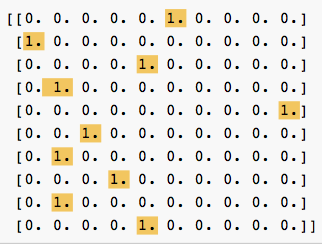
print('First x sample\n', x_train[0])
# Displays an array of 28 arrays, each containing 28 gray-scale values between 0 and 255
# Plot first x sample
plt.imshow(x_train[0])
plt.show()

# Inspect y data
print('y_train shape: ', y_train.shape)
# Displays (60000,)
print('First 10 y_train elements:', y_train[:10])
# Displays [5 0 4 1 9 2 1 3 1 4]

You have 60,000 28×28-pixel training samples and 10,000 validation samples. The first training sample is an array of 28 arrays, each containing 28 gray-scale values between 0 and 255. Looking at the non-zero values, you can see a shape like the digit 5.

Sure enough, the plt code shows the first training sample is a handwritten 5:

The y data is a 60000-element array containing the correct classifications of the training samples: the first training sample is 5, the next is 0, and so on.

Set Input & Output Dimensions

Enter these two lines, and run the cell to set up the basic dimensions of the x inputs and y outputs.

img_rows, img_cols = x_train.shape[1], x_train.shape[2]
num_classes = 10

MNIST data items are 28×28-pixel images, and you want to classify each as a digit between 0 and 9.

You use x_train.shape values to set the number of image rows and columns. x_train.shape is an array of 3 elements:

0. number of data samples: 60000
1. number of rows of each data sample: 28
2. number of columns of each data sample: 28

Reshape x Data & Set Input Shape

The model needs the data in a slightly different “shape”. Enter the code below, and run it.

# Set input_shape for channels_first or channels_last
if K.image_data_format() == 'channels_first':  
    x_train = x_train.reshape(x_train.shape[0], 1, img_rows, img_cols)
    x_val = x_val.reshape(x_val.shape[0], 1, img_rows, img_cols)
    input_shape = (1, img_rows, img_cols)
else:  
    x_train = x_train.reshape(x_train.shape[0], img_rows, img_cols, 1)
    x_val = x_val.reshape(x_val.shape[0], img_rows, img_cols, 1)
    input_shape = (img_rows, img_cols, 1)

Convolutional neural networks think of images as having width, height and depth. The depth dimension is called channels, and contains color information. Gray-scale images have 1 channel; RGB images have 3 channels.

Keras backends like TensorFlow and CNTK, expect image data in either channels-last format (rows, columns, channels) or channels-first format (channels, rows, columns). The reshape function inserts the channels in the correct position.

You also set the initial input_shape with the channels at the correct end.

Inspect Reshaped x Data

Enter the code below, and run it to see how the shapes have changed.

print('x_train shape:', x_train.shape)
# x_train shape: (60000, 28, 28, 1)
print('x_val shape:', x_val.shape)
# x_val shape: (10000, 28, 28, 1)
print('input_shape:', input_shape)
# input_shape: (28, 28, 1)

TensorFlow image data format is channels-last, so x_train.shape and x_val.shape now have a new element, 1, at the end.

Convert Data Type & Normalize Values

The model needs the data values in a specific format. Enter the code below, and run it.

x_train = x_train.astype('float32')
x_val = x_val.astype('float32')
x_train /= 255
x_val /= 255

MNIST image data values are of type uint8, in the range [0, 255], but Keras needs values of type float32, in the range [0, 1].

Inspect Normalized x Data

Enter the code below, and run it to see the changes to the x data.

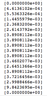
print('First x sample, normalized\n', x_train[0])
# An array of 28 arrays, each containing 28 arrays, each with one value between 0 and 1

Now each value is an array, the values are floats, and the non-zero values are between 0 and 1.

Reformat y Data

The y data is a 60000-element array containing the correct classifications of the training samples, but it’s not obvious that there are only 10 categories. Enter the code below, and run it once only to reformat the y data.

print('y_train shape: ', y_train.shape)
# (60000,)
print('First 10 y_train elements:', y_train[:10])
# [5 0 4 1 9 2 1 3 1 4]
# Convert 1-dimensional class arrays to 10-dimensional class matrices
y_train = np_utils.to_categorical(y_train, num_classes)
y_val = np_utils.to_categorical(y_val, num_classes)
print('New y_train shape: ', y_train.shape)
# (60000, 10)

y_train is a 1-dimensional array, but the model needs a 60000 x 10 matrix to represent the 10 categories. You must also make the same conversion for the 10000-element y_val array.

Inspect Reformatted y Data

Enter the code below, and run it to see how the y data has changed.

print('New y_train shape: ', y_train.shape)
# (60000, 10)
print('First 10 y_train elements, reshaped:\n', y_train[:10])
# An array of 10 arrays, each with 10 elements, 
# all zeros except at index 5, 0, 4, 1, 9 etc.

y_train is now an array of 10-element arrays, each containing all zeros except at the index that the image matches.