How To Export Blender Models to OpenGL ES: Part 2/3

Welcome back to the three-part tutorial series that teaches you how to make an awesome 3D model viewer for iOS by exporting your Blender models to OpenGL ES!

Here’s an overview of the series:

• Part 1: In the first part, you learned all about the OBJ geometry definition and file format, and used this new knowledge to create a command line tool to parse a simple Blender cube into suitable arrays for OpenGL ES. You also created a simple iOS OpenGL ES app that displayed your model.
• Part 2: You are here! Get ready to learn about the MTL material definition and file format, which you’ll use to add Blender materials (i.e. colors, textures, and lighting properties that you can assign to a portion of a model) to your cube.
• Part 3: In the final part, you’ll implement a simple lighting model for your 3D scene by writing your own OpenGL ES shaders!

Without further ado, it’s time to implement some materials!

Getting Started

First, download the starter pack for this second part of the series. Below is a quick overview of each component — you’ll find more information in their dedicated tutorial sections later on. Just as in Part 1, the contents are grouped as such:

• /Blender/: This folder contains your Blender scene (cube.blend). It’s the same cube from Part 1, but with the single cube texture replaced by different materials for each face of the cube.
• /Code/: Here you’ll find the Xcode projects for your command line tool (blender2opengles) and your iOS app (GLBlender2). The command line tool is exactly the same project from Part 1, with no modifications (minus the source and product files). The iOS app is a textureless version of GLBlender1 from Part 1. All model resources have been removed, too.
• /Resources/: This folder will contain all of your model’s files required by OpenGL ES. It’s empty for now.

Once again, I recommend you keep your directory organized as such for easy navigation.

A Fancy Blender Cube

Launch Blender and open cube.blend. Your scene should look something like this:

You’ll see the same cube from Part 1, but if you navigate the scene, you’ll notice that the cube’s shading changes with your viewing angle—for instance, the red and blue faces on the “side” of the cube maintain the same flat colors no matter your viewing angle, but the face on the top varies from shiny to dark, with gradients within the face. This is due to defining the cube with something new: material properties. So long, mere texture!

Diffuse Reflection and Specular Reflection

The reason you’re seeing this differing shading effect is due to the differing material properties of each face. Whereas a texture is like a bitmap image layered onto an object’s surface—often to provide the appearance of detailed physical texture—you can think of a material property as defining the object’s physical material in terms of how that material interacts with light.

In this tutorial, you’ll learn to implement the two most fundamental material properties, which very roughly correspond to matteness and shininess. These properties are named after two forms of reflection that create their appearance:

• Diffuse Reflection: Technically, this refers to the distributed scattering of light on a surface. More informally, this is just the reflection that lets you see things around you: when light hits an object, the light bounces off in every direction, including into your eye, which is why you can see the object. This effect also creates the perceived color of a surface when it’s illuminated by pure white light—for example, blue paint reflects blue light. In short, it’s the intrinsic color of an object.
• Specular Reflection: This refers to the focused reflection of light off a surface, in a single direction. Mirrors exhibit perfectly specular reflection, redirecting all incoming light exactly, depending on its incoming angle. However, most specular surfaces distort/absorb light differently depending on the angle, which leads to an artifact known as specular highlight on a surface—otherwise known as a shiny point.

In the real world, both properties have deep mathematical/physical models associated with them. In computer graphics, people have developed many popular algorithms that mimic these natural effects in a simple and effective way. You’ll be implementing a simplified version in Part 3, but if you’re interested in the complex physics at play, you can read more here and here.

In Blender, you can adjust your lamp properties to render diffuse and/or specular shading, as shown below:

Try turning on only diffuse reflection, and then only specular reflection, and navigating the scene to acquire some intuition for these concepts.

Blender Materials

Blender renders materials quite nicely and has many adjustable properties. You’ll implement a much simpler material shader in Part 3, but you’ll definitely carry across the diffuse and specular colors of each face. Here’s what a material looks like up close in Blender:

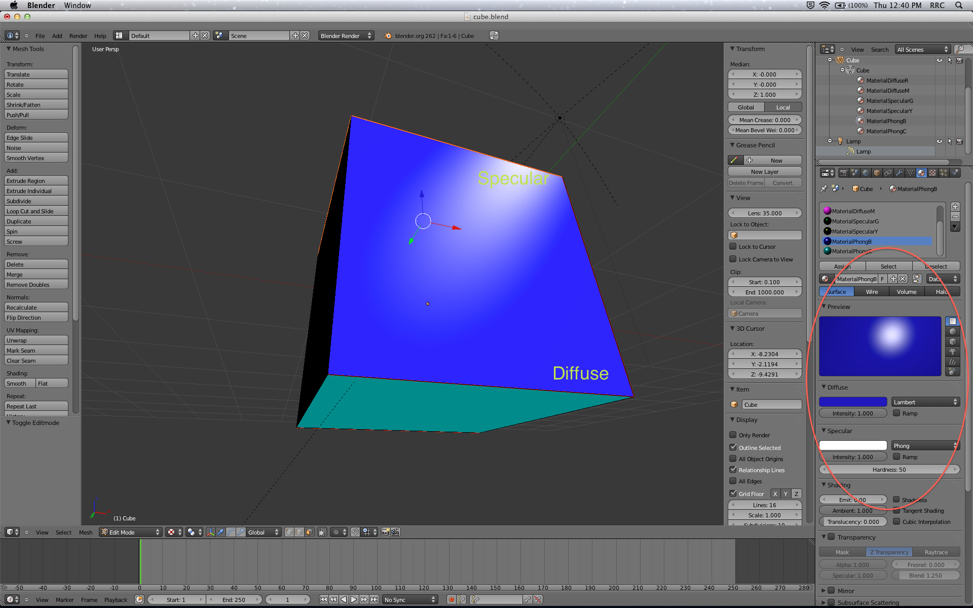
To see a flat materials preview in Blender like in the above screenshot, first, in the top-right panel—the scene outline—look under the Cube nodes and select the checkerboard-in-circle Materials icon labeled MaterialsPhongB. Then in the middle-right panel, the Properties window, look to the header of buttons, select the Materials button again and choose the material MaterialsPhongB from the list. Finally, in the Preview window, select Flat XY Plane as the type of preview.

Your scene already has predefined materials for each of the six faces. The image below shows what they look like rendered on a sphere and on Suzanne:

Let’s go over the properties for each material:

1. MaterialDiffuseR: Diffuse only (red).
2. MaterialDiffuseM: Diffuse only (magenta).
3. MaterialSpecularG: Specular only (green).
4. MaterialSpecularY: Specular only (yellow).
5. MaterialPhongB: Diffuse (blue) and specular (white).
6. MaterialPhongC: Diffuse (cyan) and specular (white).

You could use MaterialDiffuseR and MaterialDiffuseM to simulate matte surfaces like felt or cardboard, while you could use MaterialSpecularG and MaterialSpecularY to simulate shiny objects like silverware or rims. MaterialPhongB and MaterialPhongC lie between both extremes and you could use them to create a ceramic or marble appearance.

In case you’re wondering, the word Phong in the last two material names is not an arbitrary choice. It’s shorthand for the Phong reflection model, a simple lighting model that combines diffuse and specular colors. You’ll implement one in Part 3! :]

The MTL File Format

The Material Template Library (.mtl) definition describes a list of materials referenced by the geometry of an OBJ file, specifically its faces. While OBJ and MTL files go hand-in-hand, be aware that there are other popular ways to reference materials, such as mapping.

Nonetheless, now that you know all about OBJ files, you’ll have an easy time analyzing and parsing an MTL file. Plus, working with MTL is a great way to better understand the back-end of computer graphics and, later on, implement a neat shader.

An OBJ file linked to an MTL file will reference materials by name. The MTL file lists the properties of these materials with many possible attributes, but you’ll only be implementing diffuse and specular colors. You know something about these already, so let’s get to exporting!

Exporting an MTL File From Blender

MTL files are exported along with OBJ files, so many of the steps below are repeated from Part 1, but they’re worth a second walkthrough.

In Blender, with cube.blend open, go to File\Export\Wavefront (.obj). An export screen with many options will appear. Check the following boxes:

• Include Normals
• Include UVs
• Write Materials
• Triangulate Faces

Uncheck all other boxes and leave the remaining fields in their default state. Name your file cube.obj and click Export OBJ. Your materials will be exported as cube.mtl automatically. You may export or copy your newly-minted OBJ and MTL files to your /Resources/ folder if you wish.

Your material-laden cube is ready! That’s all you need from Blender for now, so you may close the application.

Analyzing Your MTL File

Using a text editor like TextEdit, open cube.obj. Its contents should look like this, possibly with some irrelevant differences due to floating point imprecision or a different order to the lines.

All the geometry components (v, vt, vn, f) will be the same as in Part 1. There is a new line towards the top of the file that looks like this:

mtllib cube.mtl

This is the reference to your MTL file, cube.mtl. That’s simple enough. If you scroll down to the end of the file, you’ll see a more interesting set of lines:

usemtl MaterialPhongC
f 1/5/6 2/8/6 3/9/6
f 1/5/6 3/9/6 4/3/6

This is a reference to the material MaterialPhongC in your linked MTL file. The material is attached to all the faces listed below the usemtl declaration—in this case, two faces.

Let’s follow this reference. Open cube.mtl in the same text editor. Its contents should look like this.

As mentioned earlier, in this tutorial you’ll only be implementing diffuse and specular colors. Using MaterialPhongC as an example again, let’s examine the relevant lines in cube.mtl:

newmtl MaterialPhongC
Kd 0.000000 0.500000 0.500000
Ks 1.000000 1.000000 1.000000

In cube.blend, MaterialPhongC is a cyan surface with a white highlight. In your MTL file, the following lines represent this material:

• Name (newmtl): The name of the material (referenced in your OBJ file).
• Diffuse color (Kd): The diffuse color of your material, in RGB color mode, with each channel ranging from 0.0 to 1.0. In this case, it’s the dark cyan: color r=0.0, g=0.5, b=0.5.
• Specular color (Ks): The specular color of your material, defined as above. In this case, it’s a pure white color: r=1.0, g=1.0, b=1.0.

That’s all you need to know about MTL files for this tutorial! You’re ready to extend your command line tool, so feel free to take a break before you start coding.

Building Your MTL to OpenGL ES Tool

Before you begin, locate your command line tool project directory using Finder (/Code/blender2opengles/) and copy your exported model files, cube.obj and cube.mtl, into the folder named source.

Using Xcode, open the blender2opengles project included in the starter kit for this part of the tutorial. As mentioned before, this is exactly the same project from Part 1, with no modifications.

Build and run your project. As expected, cube.h and cube.c are written to your directory (/Code/blender2opengles/product).

You’ll be writing to console many times before you write to a file, so for now comment out the following lines in main()—you’ll use these later:

// Save for later...
    
/*
// Write H file
writeH(filepathH, nameOBJ, model);
    
// Write C file
writeCvertices(filepathC, nameOBJ, model);
writeCpositions(filepathC, nameOBJ, model, faces, positions);
writeCtexels(filepathC, nameOBJ, model, faces, texels);
writeCnormals(filepathC, nameOBJ, model, faces, normals);
*/

Add the following line to the beginning of main(), amongst the other file path definitions:

string filepathMTL = "source/" + nameOBJ + ".mtl";

This will be a handy reference to your MTL file.

In Part 1 you created a useful data structure, Model, to represent your model’s geometry. You’re now enhancing your model with materials, so it would be very useful to have a field for the number of materials. At the top of main.cpp, add the following line as the last member within the typedef for the struct Model:

int materials;

That’s a pretty easy setup for your materials, so let’s move on.

The Material Info

It’s time to write a function to read your MTL file. Add the following function definition to main.cpp, above main():

// 1
int getMTLinfo(string fp)
{
    // 2
    int m = 0;
    
    // 3
    // Open MTL file
    ifstream inMTL;
    inMTL.open(fp);
    if(!inMTL.good())
    {
        cout << "ERROR OPENING MTL FILE" << endl;
        exit(1);
    }
    
    // 4
    // Read MTL file
    while(!inMTL.eof())
    {
        // 5
        string line;
        getline(inMTL, line);
        string type = line.substr(0,2);
        
        if(type.compare("ne") == 0)
            m++;
    }
    
    // 6
    // Close MTL file
    inMTL.close();
    
    // 7
    return m;
}

This method should be very familiar since it’s almost an exact copy of getOBJInfo() from Part 1. Here’s a quick refresher of what’s happening:

1. fp is the path of your MTL file.
2. m is a counter for your materials.
3. ifstream opens your MTL file for reading (input).
4. You read your MTL file from start to finish.
5. Each material declaration begins with the identifier newmtl, which is the only identifier in the MTL file that begins with “ne”. Therefore, the parser examines each line for this two-character token and increases the material counter m whenever it finds a match.
6. You close your MTL file.
7. You return your material counter, m.

You’ll now verify the number of materials returned. Add the following lines to main(), right after you initialize your model by calling getOBJinfo():

model.materials = getMTLinfo(filepathMTL);
cout << "Materials: " << model.materials << endl;

Build and run! You already know that you have six materials and now your program knows, too. :]

The Material Data

With your materials counted, you’ll now use this information to create arrays for their names, diffuse colors and specular colors. Add the following lines to main(), just after your geometry arrays and before your call to extractOBJdata:

string* materials = new string[model.materials];    // Name
float diffuses[model.materials][3];                 // RGB
float speculars[model.materials][3];                // RGB

materials stores a string for each material name, as spelled out in your MTL file and referenced in your OBJ file. diffuses[][3] and speculars[][3] both store three floats, one for each color channel in an RGB representation.

Now you’ll parse the material data from the MTL file into these arrays. Add the following function above main():

void extractMTLdata(string fp, string* materials, float diffuses[][3], float speculars[][3])
{
    // Counters
    int m = 0;
    int d = 0;
    int s = 0;
    
    // Open MTL file
    ifstream inMTL;
    inMTL.open(fp);
    if(!inMTL.good())
    {
        cout << "ERROR OPENING MTL FILE" << endl;
        exit(1);
    }
    
    // Read MTL file
    while(!inMTL.eof())
    {
        string line;
        getline(inMTL, line);
        string type = line.substr(0,2);
        
        // Names
        if(type.compare("ne") == 0)
        {
            // 1
            // Extract token
            string l = "newmtl ";
            materials[m] = line.substr(l.size());
            m++;
        }
        
        // 2
        // Diffuses
        else if(type.compare("Kd") == 0)
        {
            // Implementation challenge!
        }
        
        // 3
        // Speculars
        else if(type.compare("Ks") == 0)
        {
            // Implementation challenge!
        }
    }
    
    // Close MTL file
    inMTL.close();
}

Once again, this should be very familiar, but this time I’ll only introduce the new code and let you implement the rest! (Challenge accepted?):

1. As you know, the code identifies a material with the token newmtl. It then extracts the next token within the current line (after the white space) by using the function substr and discarding the string prefix “newmtl ”. The result is the material name, stored in materials.
2. Here, try implementing the code to extract the RGB data of diffuse colors into the array diffuses[][3], using d as a counter.
3. Here, try doing the same as above but for specular colors, using speculars[][3] and s.

Give it a shot! If you’re stuck or want to verify your implementation, check the solution below.

Hint: The code for this challenge is virtually identical to the parsing for positions[][3] in the function extractOBJdata() from Part 1.

[spoiler title="Parsing Materials"]

// Diffuses
else if(type.compare("Kd") == 0)
{
    // Copy line for parsing
    char* l = new char[line.size()+1];
    memcpy(l, line.c_str(), line.size()+1);
            
    // Extract tokens
    strtok(l, " ");
    for(int i=0; i<3; i++)
        diffuses[d][i] = atof(strtok(NULL, " "));
            
    // Wrap up
    delete[] l;
    d++;
}
        
// Speculars
else if(type.compare("Ks") == 0)
{
    char* l = new char[line.size()+1];
    memcpy(l, line.c_str(), line.size()+1);
            
    strtok(l, " ");
    for(int i=0; i<3; i++)
        speculars[s][i] = atof(strtok(NULL, " "));
            
    delete[] l;
    s++;
}

[/spoiler]

Three cheers for completing the challenge! Or copying the code—that works, too. :]

To see your results, add the following lines to main(), right after the call to extractOBJdata():

extractMTLdata(filepathMTL, materials, diffuses, speculars);
cout << "Name1: " << materials[0] << endl;
cout << "Kd1: " << diffuses[0][0] << "r " << diffuses[0][1] << "g " << diffuses[0][2] << "b " << endl;
cout << "Ks1: " << speculars[0][0] << "r " << speculars[0][1] << "g " << speculars[0][2] << "b " << endl;

Build and run! The console now shows the data for the first material in your MTL file, MaterialDiffuseM.

Good job—you’ve successfully parsed your MTL file!

Pairing Your Materials to Your Geometry

You’re not quite done with the materials yet. You have their data but still don’t know which faces they’re attached to. For this, you’ll have to refer back to your OBJ file.

First, inside main(), increase your faces[model.faces][9] array by 1 to store 10 integers. Your new line should look like this:

int faces[model.faces][10];                         // PTN PTN PTN M

This change causes Xcode to flag a new error for you at the call to extractOBJdata(), because faces[][10] doesn’t match the function parameter. For now, remove this function call completely; you’ll add it again shortly.

This new storage unit will be a reference to the material appended to each face, just as the OBJ file sorts faces by material. extractOBJdata() requires a major facelift, so replace your current function with the following:

// 1
void extractOBJdata(string fp, float positions[][3], float texels[][2], float normals[][3], int faces[][10], string* materials, int m)
{
    // Counters
    int p = 0;
    int t = 0;
    int n = 0;
    int f = 0;
    
    // 2
    // Index
    int mtl = 0;
    
    // Open OBJ file
    ifstream inOBJ;
    inOBJ.open(fp);
    if(!inOBJ.good())
    {
        cout << "ERROR OPENING OBJ FILE" << endl;
        exit(1);
    }
    
    // Read OBJ file
    while(!inOBJ.eof())
    {
        string line;
        getline(inOBJ, line);
        string type = line.substr(0,2);
        
        // 3
        // Material
        if(type.compare("us") == 0)
        {
            // 4
            // Extract token
            string l = "usemtl ";
            string material = line.substr(l.size());
            
            for(int i=0; i<m; i++)
            {
                // 5
                if(material.compare(materials[i]) == 0)
                    mtl = i;
            }
        }
        
        // Positions
        if(type.compare("v ") == 0)
        {
            // Copy line for parsing
            char* l = new char[line.size()+1];
            memcpy(l, line.c_str(), line.size()+1);
            
            // Extract tokens
            strtok(l, " ");
            for(int i=0; i<3; i++)
                positions[p][i] = atof(strtok(NULL, " "));
            
            // Wrap up
            delete[] l;
            p++;
        }
        
        // Texels
        else if(type.compare("vt") == 0)
        {
            char* l = new char[line.size()+1];
            memcpy(l, line.c_str(), line.size()+1);
            
            strtok(l, " ");
            for(int i=0; i<2; i++)
                texels[t][i] = atof(strtok(NULL, " "));
            
            delete[] l;
            t++;
        }
        
        // Normals
        else if(type.compare("vn") == 0)
        {
            char* l = new char[line.size()+1];
            memcpy(l, line.c_str(), line.size()+1);
            
            strtok(l, " ");
            for(int i=0; i<3; i++)
                normals[n][i] = atof(strtok(NULL, " "));
            
            delete[] l;
            n++;
        }
        
        // Faces
        else if(type.compare("f ") == 0)
        {
            char* l = new char[line.size()+1];
            memcpy(l, line.c_str(), line.size()+1);
            
            strtok(l, " ");
            for(int i=0; i<9; i++)
                faces[f][i] = atof(strtok(NULL, " /"));
            
            // 6
            // Append material
            faces[f][9] = mtl;
            
            delete[] l;
            f++;
        }
    }
    
    // Close OBJ file
    inOBJ.close();
}

That’s a big block of code (sorry!), but you’ve seen and implemented most of it before so it shouldn’t be too scary. Let’s go over the changes:

1. You’ve updated the method signature to account for the new faces[][10] array. You are also now passing materials to check your list of material names and m to loop through said list.
2. mtl is the index of a material in materials.
3. As you know, the token usemtl references a material. In an OBJ file, a comparison to the two-character token “us” is sufficient to identify this reference.
4. Just as in extractMTLdata(), you extract the material name by using the function substr and discarding the string prefix "usemtl ".
5. You then compare this material name to each material in materials, as parsed from the MTL file. Unfortunately, the materials/faces in the OBJ file are not organized in the same order of appearance as in the MTL file—hence this approach. You store the matched material as an index to materials in mtl.
6. You then append mtl to faces[f][9].

See? It’s not too bad after all.

Run your function and print out your results by adding the following lines to main(), after your call to extractMTLdata():

extractOBJdata(filepathOBJ, positions, texels, normals, faces, materials, model.materials);
    
cout << "Material References" << endl;
for(int i=0; i<model.faces; i++)
{
    int m = faces[i][9];
    cout << "F" << i << "m: " << materials[m] << endl;
}

Build and run! The console will tell you which material each face uses. Make sure the output matches your cube.obj file.

Now you’ve parsed your materials properly—nice one!

Writing the Header File (.h)

Your new header file will be very similar to the one you wrote in Part 1 and the new material data will follow the same style. Locate the function writeH() and add the following line at the end of your statistics set:

outH << "// Materials: " << model.materials << endl;

This line simply adds useful statistics comments to your header file, for your reference.

Next, add the following lines at the end of your declarations set:

// 1
outH << "const int " << name << "Materials;" << endl;
outH << "const int " << name << "Firsts[" << model.materials << "];" << endl;
outH << "const int " << name << "Counts[" << model.materials << "];" << endl;
outH << endl;
    
// 2
outH << "const float " << name << "Diffuses[" << model.materials << "]" << "[" << 3 << "];" << endl;
outH << "const float " << name << "Speculars[" << model.materials << "]" << "[" << 3 << "];" << endl;
outH << endl;

Let’s analyze these snippets separately:

1. In Part 1 of this tutorial series, OpenGL ES batch-processed all 36 vertices of your cube with glDrawArrays(). If you look at the docs and expand this function, you’ll notice the full set of parameters is glDrawArrays(GLenum mode, GLint first, GLsizei count). Now that you’re adding materials to your cube, you’ll need to render your cube by stages, according to faces grouped by materials. first will be the starting vertex of each face group and count will be the number of vertices to draw for each material.
2. This second set of statements should look a lot more familiar. Here you declare the arrays to store the actual material data, with each array tailor-made to fit the exact number of materials for the model, with three RGB channels for diffuse and specular colors.

Turn back to main() and uncomment the following line:

writeH(filepathH, nameOBJ, model);

Build and run! Using Finder, locate your new H file (/Code/blender2opengles/product/cube.h) and open it in Xcode. It should look like this:

// This is a .h file for the model: cube

// Positions: 8
// Texels: 14
// Normals: 6
// Faces: 12
// Vertices: 36
// Materials: 6

const int cubeVertices;
const float cubePositions[108];
const float cubeTexels[72];
const float cubeNormals[108];

const int cubeMaterials;
const int cubeFirsts[6];
const int cubeCounts[6];

const float cubeDiffuses[6][3];
const float cubeSpeculars[6][3];

Your header file is all set—way to fly through that one!

Writing The Implementation File (.c)

First, let’s do some housekeeping. Uncomment the following lines in main():

writeCvertices(filepathC, nameOBJ, model);
writeCpositions(filepathC, nameOBJ, model, faces, positions);
writeCtexels(filepathC, nameOBJ, model, faces, texels);
writeCnormals(filepathC, nameOBJ, model, faces, normals);

Xcode flags a few errors here because there’s a mismatch in the function parameters. Find the functions writeCpositions(), writeCtexels() and writeCnormals() and change their respective function signatures to:

void writeCpositions(string fp, string name, Model model, int faces[][10], float positions[][3])

void writeCtexels(string fp, string name, Model model, int faces[][10], float texels[][2])

void writeCnormals(string fp, string name, Model model, int faces[][10], float normals[][3])

Xcode is happy with these changes because they account for the new faces[][10] array.

Now your generated H file includes declarations of an array of cubeFirsts and an array of cubeCounts for glDrawArrays(). But there are no corresponding definitions in the generated C file yet. Let’s fix that.

Add the following lines to main(), before you call the functions to write your C file:

int firsts[model.materials];	// Starting vertex
int counts[model.materials];	// Number of vertices

Then, add counts[] as a parameter to the function call to writeCPositions(), like so:

writeCpositions(filepathC, nameOBJ, model, faces, positions, counts);

And change the function signature to:

void writeCpositions(string fp, string name, Model model, int faces[][10], float positions[][3], int counts[])

You’re going to get through this function first before you focus on the rest of the implementation file, since it’s slightly more complicated. The file handling remains the same, but the order in which you write the vertex positions is changing, so you’ll make all modifications to the for loop of writeCPositions(), shown below:

for(int i=0; i<model.faces; i++)
{
    int vA = faces[i][0] - 1;
    int vB = faces[i][3] - 1;
    int vC = faces[i][6] - 1;
        
    outC << positions[vA][0] << ", " << positions[vA][1] << ", " << positions[vA][2] << ", " << endl;
    outC << positions[vB][0] << ", " << positions[vB][1] << ", " << positions[vB][2] << ", " << endl;
    outC << positions[vC][0] << ", " << positions[vC][1] << ", " << positions[vC][2] << ", " << endl;
}

Replace said for loop with the following:

// 1
for(int j=0; j<model.materials; j++)
{
    counts[j] = 0;
        
    for(int i=0; i<model.faces; i++)
    {
        // 2
        if(faces[i][9] == j)
        {
            int vA = faces[i][0] - 1;
            int vB = faces[i][3] - 1;
            int vC = faces[i][6] - 1;
                
            outC << positions[vA][0] << ", " << positions[vA][1] << ", " << positions[vA][2] << ", " << endl;
            outC << positions[vB][0] << ", " << positions[vB][1] << ", " << positions[vB][2] << ", " << endl;
            outC << positions[vC][0] << ", " << positions[vC][1] << ", " << positions[vC][2] << ", " << endl;
                
            // 3
            counts[j] += 3;

	    // 4
            cout << "usemtl " << faces[i][9]+1 << endl;
        }
    }
}

In this instance, it’s a lot easier to show you the changes than to explain what to do step-by-step, but it’s pretty straightforward once you analyze it:

1. The original loop is nested inside another for loop, since model faces are grouped according to their material for easy rendering.
2. If there is a match between the face material reference faces[i][9] and the current material index j, then you write the current face to the material file.
3. When this happens, the vertex count, counts[], of the material index j increases by 3 vertices (triangular face).
4. This is a temporary log to show your algorithm in action. It’s difficult to appreciate the changes in your C file at the moment, and I don’t want to over-comment it either.

Build and run. There’s nothing too exciting just yet, but the console shows the materials written in order, each used in two faces as expected. You may remove the cout statement.

Challenge time! This one should be easy, since you’ll modify the functions writeCtexels() and writeCnormals() as above, but without having to worry about counts[].

Hint: There’s no need to change the function signature—just the for loop inside each.

[spoiler title="The Small Refactor"]
For writeCtexels():

// Texels
for(int j=0; j<model.materials; j++)
{
    for(int i=0; i<model.faces; i++)
    {
        if(faces[i][9] == j)
        {
            int vtA = faces[i][1] - 1;
            int vtB = faces[i][4] - 1;
            int vtC = faces[i][7] - 1;
                
            outC << texels[vtA][0] << ", " << texels[vtA][1] << ", " << endl;
            outC << texels[vtB][0] << ", " << texels[vtB][1] << ", " << endl;
            outC << texels[vtC][0] << ", " << texels[vtC][1] << ", " << endl;
        }
    }
}

For writeCnormals():

// Normals
for(int j=0; j<model.materials; j++)
{
    for(int i=0; i<model.faces; i++)
    {
        if(faces[i][9] == j)
        {
            int vnA = faces[i][2] - 1;
            int vnB = faces[i][5] - 1;
            int vnC = faces[i][8] - 1;
                
            outC << normals[vnA][0] << ", " << normals[vnA][1] << ", " << normals[vnA][2] << ", " << endl;
            outC << normals[vnB][0] << ", " << normals[vnB][1] << ", " << normals[vnB][2] << ", " << endl;
            outC << normals[vnC][0] << ", " << normals[vnC][1] << ", " << normals[vnC][2] << ", " << endl;
        }
    }
}

[/spoiler]

And just like that, you’ve restructured your OBJ data!

In Part 1, I mentioned the benefits of modules and then you implemented separate functions for each attribute array. You’ll be doing the same in this part, too, starting with the model’s firsts[] and counts[].

Add the following function to main.cpp, just above main():

void writeCmaterials(string fp, string name, Model model, int firsts[], int counts[])
{
    // Append C file
    ofstream outC;
    outC.open(fp, ios::app);
    
    // Materials
    outC << "const int " << name << "Materials = " << model.materials << ";" << endl;
    outC << endl;
    
    // Firsts
    outC << "const int " << name << "Firsts[" << model.materials << "] = " << endl;
    outC << "{" << endl;
    for(int i=0; i<model.materials; i++)
    {
        // 1
        if(i == 0)
            firsts[i] = 0;
        else
            firsts[i] = firsts[i-1]+counts[i-1];
        
        // 2
        outC << firsts[i] << "," << endl;
    }
    outC << "};" << endl;
    outC << endl;
    
    // Counts
    outC << "const int " << name << "Counts[" << model.materials << "] = " << endl;
    outC << "{" << endl;
    for(int i=0; i<model.materials; i++)
    {
        // 3
        outC << counts[i] << "," << endl;
    }
    outC << "};" << endl;
    outC << endl;
    
    // Close C file
    outC.close();
}

The majority of this function should be standard file I/O for you by now, so let’s just go over the new lines pertaining to firsts[] and counts[]:

1. You’ve created an array of firsts but you haven’t stored any data in it. Luckily, you can do this as you write out your C file. You’re about to render the first group of faces. If you’re writing data for the first material, then the starting vertex is 0. For all additional materials, the starting vertex is equal to the first vertex of the previous material plus the number of vertices drawn.
2. So, once you’ve determined the result you simply write it to your C file.
3. You filled in the data for counts[] earlier, so another simple write suffices here.

Next, add the following line to the end of main():

writeCmaterials(filepathC, nameOBJ, model, firsts, counts);

Build and run! Using Finder, locate your new C file (/Code/blender2opengles/product/cube.c) and open it in Xcode. The new code at the end of the file should look like this:

const int cubeMaterials = 6;

const int cubeFirsts[6] = 
{
0,
6,
12,
18,
24,
30,
};

const int cubeCounts[6] = 
{
6,
6,
6,
6,
6,
6,
};

Your hard work has paid off! And there’s more good news—you’re almost done. It’s time to implement your model’s diffuse and specular colors.

Add the following function above main():

void writeCdiffuses(string fp, string name, Model model, float diffuses[][3])
{
    // Append C file
    ofstream outC;
    outC.open(fp, ios::app);
    
    // Diffuses
    outC << "const float " << name << "Diffuses[" << model.materials << "][3] = " << endl;
    outC << "{" << endl;
    for(int i=0; i<model.materials; i++)
    {
        outC << diffuses[i][0] << ", " << diffuses[i][1] << ", " << diffuses[i][2] << ", " << endl;
    }
    outC << "};" << endl;
    outC << endl;
    
    // Close C file
    outC.close();
}

You should know exactly what’s going on here—you’re simply writing out the RGB diffuse color data of each material. This makes your next challenge very easy... do the same for your specular colors!

Hint: Nope, no hint this time. That would make it far too easy. :]

[spoiler title="Time to Shine"]

void writeCspeculars(string fp, string name, Model model, float speculars[][3])
{
    // Append C file
    ofstream outC;
    outC.open(fp, ios::app);
    
    // Speculars
    outC << "const float " << name << "Speculars[" << model.materials << "][3] = " << endl;
    outC << "{" << endl;
    for(int i=0; i<model.materials; i++)
    {
        outC << speculars[i][0] << ", " << speculars[i][1] << ", " << speculars[i][2] << ", " << endl;
    }
    outC << "};" << endl;
    outC << endl;
    
    // Close C file
    outC.close();
}

[/spoiler]

Finally, add the following lines at the end of main():

writeCdiffuses(filepathC, nameOBJ, model, diffuses);
writeCspeculars(filepathC, nameOBJ, model, speculars);

Build and run! Open cube.c in Xcode and check out your finalized implementation file, which should look like this.

Congratulations, your blender2opengles tool is complete! Your fancy blender model is all set and your materials are ready to shine. Unless they are diffuse, that is…

Copy your files cube.h and cube.c into your /Resources/ folder and take a well-deserved break before you hit the app.

Enhancing Your Model Viewer iOS App

Open your GLBlender2 project in Xcode and add your enhanced resources to your project: cube.h and cube.c. You may also add cube.obj and cube.mtl, but it’s not necessary.

Build and run! You should see your same cube from Part 1, but without a texture. This may not seem exciting, but it’s very important to know that you haven’t compromised your model’s geometry by adding materials.

GLKBaseEffect Materials

Now that you know a lot more about materials and your model is not textured, I’m sure you can appreciate the shading of the cube. The default material properties for GLKBaseEffect, defined by GLKEffectPropertyMaterial, are:

// Properties					// Default Values
GLKVector4		ambientColor;         	// { 0.2, 0.2, 0.2, 1.0}
GLKVector4       	diffuseColor;           // { 0.8, 0.8, 0.8, 1.0}
GLKVector4       	specularColor;          // { 0.0, 0.0, 0.0, 1.0}
GLKVector4       	emissiveColor;          // { 0.0, 0.0, 0.0, 1.0}
GLfloat          	shininess;              // 0.0

That’s exactly what you’re seeing on your cube—a grayish surface. The fourth value is alpha in RGBA mode.

Let’s play around with these parameters, shall we?

Open MainViewController.m and scroll down to the function glkView:drawInRect:. Make sure your call to prepareToDraw happens just before your call to glDrawArrays(). Then, just before those two lines, add the following piece of code:

// Set material
self.effect.material.diffuseColor = GLKVector4Make(0.8f, 0.0f, 0.0f, 1.0f);
self.effect.material.specularColor = GLKVector4Make(0.0f, 0.0f, 0.2f, 1.0f);

In case you’re feeling a bit lost, the complete function should look like this:

- (void)glkView:(GLKView *)view drawInRect:(CGRect)rect
{
    glClear(GL_COLOR_BUFFER_BIT);
    
    // Set matrices
    [self setMatrices];
    
    // Positions
    glEnableVertexAttribArray(GLKVertexAttribPosition);
    glVertexAttribPointer(GLKVertexAttribPosition, 3, GL_FLOAT, GL_FALSE, 0, cubePositions);
    
    // Normals
    glEnableVertexAttribArray(GLKVertexAttribNormal);
    glVertexAttribPointer(GLKVertexAttribNormal, 3, GL_FLOAT, GL_FALSE, 0, cubeNormals);
    
    // Set material
    self.effect.material.diffuseColor = GLKVector4Make(0.8f, 0.0f, 0.0f, 1.0f);
    self.effect.material.specularColor = GLKVector4Make(0.0f, 0.0f, 0.2f, 1.0f);
    
    // Prepare effect
    [self.effect prepareToDraw];
    
    // Draw Model
    glDrawArrays(GL_TRIANGLES, 0, cubeVertices);
}

Build and run! Now you have a bold red cube (diffuse) with a faint blue glow (specular).

Let’s make things more interesting by adding two materials to this cube.

First, draw half of your vertices by changing glDrawArrays() to:

glDrawArrays(GL_TRIANGLES, 0, cubeVertices/2);

Then, add a new material and draw the other half of the cube by adding the following lines to the end of glkView:drawInRect::

// Change material
self.effect.material.diffuseColor = GLKVector4Make(0.0f, 0.9f, 0.0f, 1.0f);
self.effect.material.specularColor = GLKVector4Make(0.1f, 0.1f, 0.1f, 1.0f);
    
// Prepare effect again
[self.effect prepareToDraw];
    
// Draw 2nd half of model
glDrawArrays(GL_TRIANGLES, cubeVertices/2, cubeVertices/2);

Now you’re rendering half of your cube as an almost-matte green surface. You call prepareToDraw again because you’ve changed the effect, and then glDrawArrays() begins drawing from the previous half of the cube for another half-count of vertices.

Build and run to see the results!

I hope you’re already guessing—and are ready for—what’s about to happen next, but feel free to play around with the material properties. Just don’t stray too far...

Rendering by Parts

Instead of adding a long list of materials and drawing calls in your rendering function, let’s tidy things up with a loop.

First, delete all your calls to self.effect.material, prepareToDraw and glDrawArrays() inside glkView:drawInRect:. Then add the following lines at the bottom of said function:

// Render by parts
for(int i=0; i<cubeMaterials; i++)
{
    // Prepare effect
    [self.effect prepareToDraw];
        
    // Draw vertices
    glDrawArrays(GL_TRIANGLES, cubeFirsts[i], cubeCounts[i]);
}

Since your faces are grouped by materials, your loop should render all materials according to cubeMaterials. In your command line tool, you also determine the size of cubeFirsts[] and cubeCounts[] by the number of materials, so you won’t encounter any access errors. These two arrays work with each other, so they’re quite organized and know exactly which vertex to start drawing from and how many vertices to draw.

If you were to write out the loop (don’t actually do this), this is what it would look like:

// EXAMPLE ONLY, DO NOT IMPLEMENT
// Render by parts (i<6)
glDrawArrays(GL_TRIANGLES, 0, 6);   // i=0
glDrawArrays(GL_TRIANGLES, 6, 6);   // i=1
glDrawArrays(GL_TRIANGLES, 12, 6);  // i=2
glDrawArrays(GL_TRIANGLES, 18, 6);  // i=3
glDrawArrays(GL_TRIANGLES, 24, 6);  // i=4
glDrawArrays(GL_TRIANGLES, 30, 6);  // i=5

And that’s how your full, 36-vertex cube gets rendered! Build and run to see it with your own eyes. It should look exactly the same as the first gray cube you rendered.

Rendering Your Materials

The last step is to get your materials onto that cube! Add the following lines inside your for loop, before any of your drawing commands:

// Set material
self.effect.material.diffuseColor = GLKVector4Make(cubeDiffuses[i][0], cubeDiffuses[i][1], cubeDiffuses[i][2], 1.0f);
self.effect.material.specularColor = GLKVector4Make(cubeSpeculars[i][0], cubeSpeculars[i][1], cubeSpeculars[i][2], 1.0f);

With these two lines, you set the appropriate material properties to be attached to each face group.

Build and run! You should see a nice colorful cube now...

...but it’s not what you were expecting. The materials are correct, but MaterialPhongC is far too bright and its specular color, white, is completely overpowering its diffuse color, cyan. You can try to fix this by adjusting your scene’s lighting.

In MainViewController.m, add the following lines to createEffect, amongst your light declarations:

self.effect.light0.specularColor = GLKVector4Make(0.25f, 0.25f, 0.25f, 1.0f);
self.effect.light0.diffuseColor = GLKVector4Make(0.75f, 0.75f, 0.75f, 1.0f);

Your scene now has a lighting intensity of 25% white for specular surfaces and 75% white for diffuse surfaces.

Build and run! You’ve got your cyan back, but the scene may be too dark for your liking.

You can play around with your lights and materials, but the truth is that GLKBaseEffect has limited rendering options because it mimics the fixed-function pipeline of OpenGL ES 1.x.

Blender and other high-end graphics software tend to run sophisticated lighting algorithms by implementing shaders. You’ll learn more about these in Part 3, but essentially they are dedicated programs that allow you to develop you own lighting models and other special effects. Since OpenGL ES 2.x, the fixed-function pipeline has become a thing of the past thanks to programmable shaders, which are coded in GLSL and run on the GPU.

OpenGL ES isn’t the only API implementing a programmable, shader-based pipeline. Microsoft (Direct3D with HLSL) and Pixar (Renderman with RSL) also use this type of architecture. That’s all the more reason to learn more about shaders in Part 3. :]

Where to Go From Here?

Here is the completed project with all of the code and resources from this part of the Blender to OpenGL ES tutorial. You can also find its repository on GitHub.

Congratulations, you’ve enhanced your model viewer and knowledge of 3D graphics by handling and implementing materials! This part of the series was quite tricky, especially when parsing two separate graphics files to produce one model representation.

You should now understand the material properties of simple surfaces and know how to analyze an OBJ/MTL file pair. By now, you’re a total pro when it comes to command line tools in Xcode and really know your way around file I/O. You’ve explored GLKit a bit more and hopefully you’ve noticed the trade-off between ease of implementation and quality of rendering.

In Part 3 of this tutorial series, you’ll take a deep dive into the world of shaders and advanced OpenGL ES. You’ll learn a new programming language, GLSL, and use it to have complete control of your scene’s lighting. Even better, you'll get a new model to play around with. :]

If you have any questions, comments or suggestions, feel free to join the discussion below!