Introduction to the Visual Effect Graph
In this Visual Effect Graph tutorial, you’ll learn how to easily create complex visual effects in Unity with a node editor. By Harrison Hutcheon.
Parameter Binders
You’ll use the Blackboard to expose variables to the Unity editor and to MonoBehaviour scripts. For this effect, you want to set two positions so your particles can travel between them: A Start Position, which is the resource icon location and a Tower Position, which is the tower you’re upgrading.
Start by clicking the + icon on the Blackboard to create a new variable and selecting Vector3 from the menu. In the Inspector, name this variable StartPosition. Then repeat the same steps, naming the next variable TowerPosition.
In the Inspector, check Exposed for each variable. This gives you access to the variables outside the graph.

To access these particles in a script, call one of the visual effect’s many Set methods. For example, to set the Vector3 value, you would use:
yourVisualEffect.SetVector3("VariableName", newVector3Value);
You’ve now defined your two positions. You just need to get your particles to move between them next!
Controlling Particle Movement
To move particles from the StartPosition to the TowerPosition, you’ll construct your first VFX operation using nodes. This operation will apply a Bézier curve to the movement of the particles, extending over the lifetime of each particle.

In a large, empty space to the left of the main graph, create an Age Over Lifetime node by right-clicking the empty space and selecting Create Node ▸ Operator ▸ Attribute ▸ Age over Lifetime. Drag StartPosition and TowerPosition onto the graph underneath it.

Next, create a Sample Curve node, an Add node and a Sample Bezier node. You can easily find these nodes by typing their names in the search field at the top of the Create Node window.
Once you have the nodes, set Add to Vector3 by clicking the gear in the top-right of the node and setting both values to Vector3.

Connect the nodes in the following way:
- Connect Age Over Lifetime to the Time input of Sample Curve and connect the s output of the sample curve to the T input of Sample Bezier. This binds the the duration of the bezier curve to the lifetime of the particle.
- Connect StartPosition to the B input of Sample Bezier. This sets the initial position of the curve to the resource pool in the center of the screen.
- Connect TowerPosition to the B input of Add, and connect the output of Add to the C input of Sample Bezier. You will use this operation to create midpoint for the Bezier operation.
- Finally, connect TowerPosition to the D input of Sample Bezier. This sets the final position of the curve.
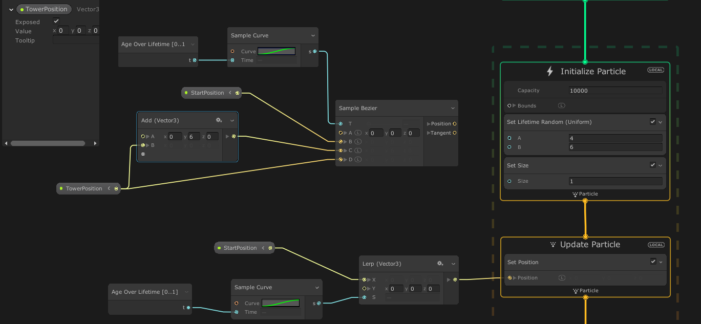
When complete, the operation as a whole should look like this:

Set the Y value of Add to 6. This creates a point above the tower to make the arc skew upwards.
Click the graph in Sample Curve and configure it with just two points on the curve. (remove the middle node). The first node will sit at (X: 0, Y: 0) and the second node should sit at (X: 0.2, Y: 1.0).

This curve ensures that each particle will reach the end of the curve during the first quarter of their total lifetime. This is necessary because later operations of this VFX Graph will take place after the particles have reached the selected tower.
To use this operation to affect the movement of each particle, you’ll have to lerp each particle’s position between StartPosition and the value calculated by this operation.
Copy the Age Over Lifetime and Sample Curve nodes and move them to the empty space below the Bézier operation.
Create a Lerp node and configure it to accept Vector3s. Leave the S value as a float.
Drag a new reference to StartPosition onto the graph, position it to the left of Lerp and connect all of the nodes as follows:
- Start Position ▸ Lerp X value.
- Sample Curve S value ▸ Lerp S value.
- Age Over Lifetime t value ▸ Sample Curve Time value.

Create a Set Position block in Update Particle and connect the output of the Lerp node to its position field.
As a quick checkpoint, your graph should look like the following:
At the moment, you could attach the Bézier operation to this Lerp, which would move the particles in an interesting way. However, you can take things a step further by adding a noise operation, which adds chaos and makes the effect more interesting. You’ll do that in the next step.
Adding Noise
Noise, in the context of computer graphics, refers to applying randomization to create a unique and unpredictable effect. For this visual effect, you’ll apply noise to the particles so they appear to buzz around while they travel to the selected tower.

Create the following nodes in the space above the Bézier operation (you may want to reposition things first to make some room):
- Random Number
- AppendVector
- Lerp (Float)
- Multiply
- Age Over Lifetime
- Sample Curve
Set the Min of Random Number to -1 and the Max to 1.
Next, create two copies of Random Number. Set the seed of each Random Number to 1, 2 and 3, respectively.
Configure AppendVector to accept three floats. You can add a new float to its values with the + icon at the bottom of the node.
Now, configure Multiply to accept a Vector3 and two floats. Rename the first float, B, to Scale and set it to 2.
Set the Y value of Lerp to 3, then set the Sample Curve to a standard upward curve.
Connect the new nodes as follows:
- Connect the 3 x Random Number nodes to AppendVector‘s A, B, and C inputs.
- Connect AppendVector‘s output to the Multiply‘s A input.
- Connect Age Over Lifetime‘s output to the Sample Curve Time input.
- Connect the output of Sample Curve to the S input on Lerp.
- Connect the Lerp output to the Multiply C input.

For your next step, you need a way to use this noise operation with the Bézier operation. So create a new Add node and configure it to accept Vector3 inputs.
Connect the output from the Multiply node and the Position output from the Sample Bézier node to input slots from the new Add node. Then connect the output from the new Add node to the second input of the Lerp node that’s connected to the Set Position block in the Update Particle Context.
You should end up with a node configuration like this (click the image to open it up in a larger view if you want to see the detail):
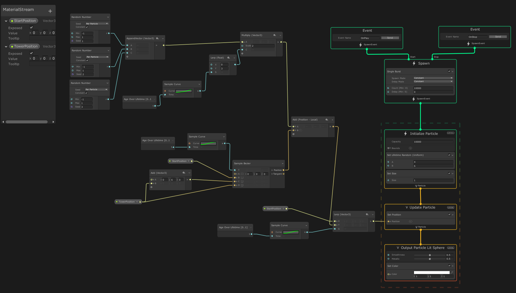
That’s it! Save your progress. Your particles will now travel to their destination in a noisy, Bézier curve formation. :]