Unreal Engine 4 Paint Filter Tutorial

As time passes, video games continue to look better and better. And in an era of video games with amazing visuals, it can be hard to make your game stand out. A way to make your game’s aesthetic more unique is to use non-photorealistic rendering.

Non-photorealistic rendering encompasses a wide range of rendering techniques. These include but are not limited to cel shading, toon outlines and cross hatching. You can even make your game look more like a painting! One of the techniques to accomplish this is Kuwahara filtering.

To implement Kuwahara filtering, you will learn how to:

• Calculate mean and variance for multiple kernels
• Output the mean of the kernel with lowest variance
• Use Sobel to find a pixel’s local orientation
• Rotate the sampling kernels based on the pixel’s local orientation

Getting Started

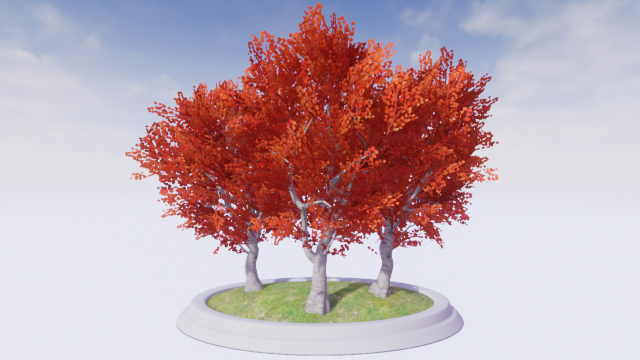
Start by downloading the materials for this tutorial (you can find a link at the top or bottom of this tutorial). Unzip it and navigate to PaintFilterStarter and open PaintFilter.uproject. You will see the following scene:

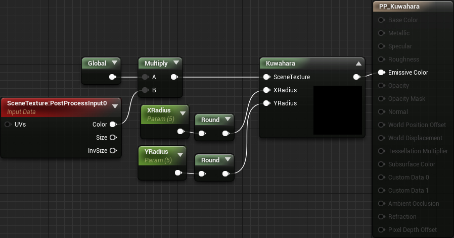
To save time, the scene already contains a Post Process Volume with PP_Kuwahara. This is the material (and its shader files) you will be editing.

To start, let’s go over what the Kuwahara filter is and how it works.

Kuwahara Filter

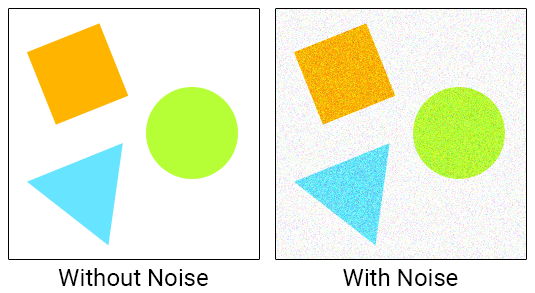
When taking photos, you may notice a grainy texture over the image. This is noise and just like the noise coming from your loud neighbors, you probably don’t want to see or hear it.

A common way to remove noise is to use a low-pass filter such as a blur. Below is the noise image after box blurring with a radius of 5.

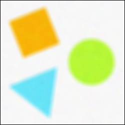
Most of the noise is now gone but all the edges have lost their hardness. If only there was a filter that could smooth the image and preserve the edges!

As you might have guessed, the Kuwahara filter meets these requirements. Let’s look at how it works.

How Kuwahara Filtering Works

Like convolution, Kuwahara filtering uses kernels but instead of using one kernel, it uses four. The kernels are arranged so that they overlap by one pixel (the current pixel). Below is an example of the kernels for a 5×5 Kuwahara filter.

First, you calculate the mean (average color) for each kernel. This essentially blurs the kernel which has the effect of smoothing out noise.

For each kernel, you also calculate the variance. This is basically a measure of how much a kernel varies in color. For example, a kernel with similar colors will have low variance. If the colors are dissimilar, the kernel will have high variance.

Finally, you find the kernel with the lowest variance and output its mean. This selection based on variance is how the Kuwahara filter preserves edges. Let’s look at a few examples.

Kuwahara Filtering Examples

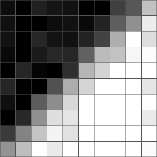
Below is a 10×10 grayscale image. You can see that there is an edge going from the bottom-left to the top-right. You can also see that some areas of the image have noise.

First, select a pixel and determine which kernel has the lowest variance. Here is a pixel near the edge and its associated kernels:

As you can see, kernels lying on the edge have varying colors. This indicates high variance and means the filter will not select them. By not selecting kernels lying on an edge, the filter avoids the problem of blurred edges.

For this pixel, the filter will select the green kernel since it is the most homogeneous. The output will then be the mean of the green kernel which is a color close to black.

Here’s another edge pixel and its kernels:

This time the yellow kernel has the least variance since it’s the only one not on the edge. So the output will be the mean of the yellow kernel which is a color close to white.

Below is a comparison between box blurring and Kuwahara filtering — each with a radius of 5.

As you can see, Kuwahara filtering does a great job at smoothing and edge preserving. In this case, the filter actually hardened the edge!

Incidentally, this edge-preserving smoothing feature can give an image a painterly look. Since brush strokes generally have hard edges and low noise, the Kuwahara filter is a great choice for converting realistic images to a painterly style.

Here is the result of running a photo through Kuwahara filters of varying size:

It looks pretty good, doesn’t it? Let’s go ahead and start creating the Kuwahara filter.

Creating the Kuwahara Filter

For this tutorial, the filter is split into two shader files: Global.usf and Kuwahara.usf. The first file will store a function to calculate a kernel’s mean and variance. The second file is the filter’s entry point and will call the aforementioned function for each kernel.

First, you will create the function to calculate mean and variance. Open the project folder in your OS and then go to the Shaders folder. Afterwards, open Global.usf. Inside, you will see the GetKernelMeanAndVariance() function.

Before you start building the function, you will need an extra parameter. Change the function’s signature to:

float4 GetKernelMeanAndVariance(float2 UV, float4 Range)

To sample in a grid, you need two for loops: one for horizontal offsets and another for vertical offsets. The first two channels of Range will contain the bounds for the horizontal loop. The second two will contain the bounds for the vertical loop. For example, if you are sampling the top-left kernel and the filter has a radius of 2, Range would be:

Range = float4(-2, 0, -2, 0);

Now it’s time to start sampling.

Sampling Pixels

First, you need to create the two for loops. Add the following inside GetKernelMeanAndVariance() (below the variables):

for (int x = Range.x; x <= Range.y; x++)
{
    for (int y = Range.z; y <= Range.w; y++)
    {
        
    }
}

This will give you all the offsets for the kernel. For example, if you are sampling the top-left kernel and the filter has a radius of 2, the offsets will range from (0, 0) to (-2, -2).

Now you need to get the color for the sample pixel. Add the following inside the inner for loop:

float2 Offset = float2(x, y) * TexelSize;
float3 PixelColor = SceneTextureLookup(UV + Offset, 14, false).rgb;

The first line will get the sample pixel’s offset and convert it to UV space. The second line will use the offset to get the sample pixel’s color.

Next, you need to calculate the mean and variance.

Calculating Mean and Variance

Figuring out the mean is easy enough. You just accumulate all the colors and then divide by the number of samples. For variance, you use the formula below where x is the sample pixel’s color:

The first thing you need to do is calculate the sums. For the mean, this is just adding the color to the Mean variable. For variance, you need to square the color before adding it to Variance. Add the following below the previous code:

Mean += PixelColor;
Variance += PixelColor * PixelColor;
Samples++;

Next, add the following below the for loops:

Mean /= Samples;
Variance = Variance / Samples - Mean * Mean;
float TotalVariance = Variance.r + Variance.g + Variance.b;
return float4(Mean.r, Mean.g, Mean.b, TotalVariance);

The first two lines will calculate the mean and variance. However, there is a problem: the variance is spread across the RGB channels. To fix this, the third line sums the channels up to give you the total variance.

Finally, the function returns the mean and variance as a float4. The mean is in the RGB channels and variance is in the A channel.

Now that you have a function to calculate the mean and variance, you need to call it for each kernel. Go back to the Shaders folder and open Kuwahara.usf. First, you need to create a few variables. Replace the code inside with the following:

float2 UV = GetDefaultSceneTextureUV(Parameters, 14);
float4 MeanAndVariance[4];
float4 Range;

Here is what each variable is for:

• UV: UV coordinates for the current pixel
• MeanAndVariance: An array to hold the mean and variance for each kernel
• Range: Used to hold the for loop bounds for the current kernel

Now you need to call GetKernelMeanAndVariance() for each kernel. To do this, add the following:

Range = float4(-XRadius, 0, -YRadius, 0);
MeanAndVariance[0] = GetKernelMeanAndVariance(UV, Range);

Range = float4(0, XRadius, -YRadius, 0);
MeanAndVariance[1] = GetKernelMeanAndVariance(UV, Range);

Range = float4(-XRadius, 0, 0, YRadius);
MeanAndVariance[2] = GetKernelMeanAndVariance(UV, Range);

Range = float4(0, XRadius, 0, YRadius);
MeanAndVariance[3] = GetKernelMeanAndVariance(UV, Range);

This will get the mean and variance for each kernel in the following order: top-left, top-right, bottom-left and then bottom-right.

Next, you need to select the kernel with lowest variance and output its mean.

Selecting Kernel With Lowest Variance

To select the kernel with lowest variance, add the following:

// 1
float3 FinalColor = MeanAndVariance[0].rgb;
float MinimumVariance = MeanAndVariance[0].a;

// 2
for (int i = 1; i < 4; i++)
{
    if (MeanAndVariance[i].a < MinimumVariance)
    {
        FinalColor = MeanAndVariance[i].rgb;
        MinimumVariance = MeanAndVariance[i].a;
    }
}

return FinalColor;

Here is what each section does:

1. Create two variables to hold the final color and minimum variance. Initialize both of these to the first kernel’s mean and variance.
2. Loop over the remaining three kernels. If the current kernel’s variance is lower than the minimum, its mean and variance become the new FinalColor and MinimumVariance. After looping, the output is FinalColor which will be the mean of the lowest variance kernel.

Go back to Unreal and navigate to Materials\PostProcess. Open PP_Kuwahara, make a dummy change and then click Apply. Go back to the main editor to see the results!

It looks pretty good but if you look closer, you can see that the image has these strange block-like areas. Here’s a few of them highlighted:

This is a side effect of using axis-aligned kernels. A way to reduce this is to use an improved version of the filter which I call the Directional Kuwahara filter.

Directional Kuwahara Filter

This filter is like the original except the kernels are now aligned with the pixel’s local orientation. Here is an example of a 3×5 kernel in the Directional Kuwahara filter:

Here, the filter determines the pixel’s orientation to be along the edge. It then rotates the entire kernel accordingly.

To calculate the local orientation, the filter does a convolution pass using Sobel. If Sobel sounds familiar to you, it’s probably because it is a popular edge detection technique. But if it’s an edge detection technique, how can you use it to get local orientation? To answer that, let’s look at how Sobel works.

How Sobel Works

Instead of one kernel, Sobel uses two.

Gx will give you the gradient in the horizontal direction. Gy will give you the gradient in the vertical direction. Let’s use the following 3×3 grayscale image as an example:

First, convolve the middle pixel with each kernel.

If you plot each value onto a 2D plane, you will see that the resulting vector points in the same direction as the edge.

To find the angle between the vector and the X-axis, you plug the gradient values into an arc tangent (atan) function. You can then use the resulting angle to rotate the kernel.

And that’s how you can use Sobel to give you a pixel’s local orientation. Let’s try it out.

Finding Local Orientation

Open Global.usf and add the following inside GetPixelAngle():

float GradientX = 0;
float GradientY = 0;
float SobelX[9] = {-1, -2, -1, 0, 0, 0, 1, 2, 1};
float SobelY[9] = {-1, 0, 1, -2, 0, 2, -1, 0, 1};
int i = 0;

Here’s what each variable is for:

• GradientX: Holds the gradient for the horizontal direction
• GradientY: Holds the gradient for the vertical direction
• SobelX: The horizontal Sobel kernel as an array
• SobelY: The vertical Sobel kernel as an array
• i: Used to access each element in SobelX and SobelY

Next, you need to perform convolution using the SobelX and SobelY kernels. Add the following:

for (int x = -1; x <= 1; x++)
{
    for (int y = -1; y <= 1; y++)
    {
        // 1
        float2 Offset = float2(x, y) * TexelSize;
        float3 PixelColor = SceneTextureLookup(UV + Offset, 14, false).rgb;
        float PixelValue = dot(PixelColor, float3(0.3,0.59,0.11));
        
        // 2
        GradientX += PixelValue * SobelX[i];
        GradientY += PixelValue * SobelY[i];
        i++;
    }
}

Here’s what each section does:

1. The first two lines will get the sample pixel’s color. The third line will then desaturate the color to convert it into a single grayscale value. This makes it easier to calculate the gradients of the image as a whole instead of getting the gradients for each color channel.
2. For both kernels, multiply the pixel’s grayscale value with the corresponding kernel element. Then add the result to the appropriate gradient variable. i will then increment to hold the index for the next kernel element.

To get the angle, you use the atan() function and plug in your gradient values. Add the following below the for loops:

return atan(GradientY / GradientX);

Now that you have a function to get a pixel’s angle, you need to somehow use it to rotate the kernel. A way to do this is to use a matrix.

What is a Matrix?

A matrix is a 2D array of numbers. For example, here is a 2×3 matrix (two rows and three columns):

By itself, a matrix doesn’t look very interesting. But the matrix’s true power reveals itself once you multiply a vector with a matrix. This will allow you to do things such as rotation and scaling (depending on the matrix). But how exactly do you create a matrix for rotation?

In a coordinate system, you will have a vector for every dimension. These are your basis vectors and they define the positive directions of your axes.

Below are a few examples of different basis vectors for a 2D coordinate system. The red arrow defines the positive X direction. The green arrow defines the positive Y direction.

To rotate a vector, you can use these basis vectors to build a rotation matrix. This is simply a matrix containing the positions of the basis vectors after rotation. For example, imagine you have a vector (orange arrow) at (1, 1).

Let’s say you want to rotate it 90 degrees clockwise. First, you rotate the basis vectors by the same amount.

Then you construct a 2×2 matrix using the new positions of the basis vectors. The first column is the red arrow’s position and the second column is the green arrow’s position. This is your rotation matrix.

Finally, you perform matrix multiplication using the orange vector and rotation matrix. The result is the new position for the orange vector.

Isn’t that cool? What’s even better is that you can use the matrix above to rotate any 2D vector 90 degrees clockwise. For the filter, this means you only need to construct the rotation matrix once for each pixel and then you can use it for the entire kernel.

Now it’s time to rotate the kernel using a rotation matrix.

Rotating the Kernel

First, you need to modify GetKernelMeanAndVariance() to accept a 2×2 matrix. This is because you will construct a rotation matrix within Kuwahara.usf and pass it in. Change the signature for GetKernelMeanAndVariance() to:

float4 GetKernelMeanAndVariance(float2 UV, float4 Range, float2x2 RotationMatrix)

Next, change the first line in the inner for loop to:

float2 Offset = mul(float2(x, y) * TexelSize, RotationMatrix);

mul() will perform matrix multiplication using the offset and RotationMatrix. This will rotate the offset around the current pixel.

Next, you need to construct the rotation matrix.

Constructing the Rotation Matrix

To construct a rotation matrix, you use the sine and cosine functions like so:

Close Global.usf and then open Kuwahara.usf. Afterwards, add the following at the bottom of the variable list:

float Angle = GetPixelAngle(UV);
float2x2 RotationMatrix = float2x2(cos(Angle), -sin(Angle), sin(Angle), cos(Angle));

The first line will calculate the angle for the current pixel. The second line will then create the rotation matrix using the angle.

Finally, you need to pass in the RotationMatrix for each kernel. Modify each call to GetKernelMeanAndVariance() like so:

GetKernelMeanAndVariance(UV, Range, RotationMatrix)

That’s all for the Directional Kuwahara! Close Kuwahara.usf and then go back to PP_Kuwahara. Make a dummy change, click Apply and then close it.

Below is a comparison between the original Kuwahara and Directional Kuwahara. Notice how the Directional Kuwahara does not have the blockiness of the original.

Where to Go From Here?

You can download the completed project using the link at the top or bottom of this tutorial.

If you’d like to learn more about the Kuwahara filter, check out the paper on Anisotropic Kuwahara filtering. The Directional Kuwahara is actually a simplified version of the filter presented in the paper.

Using your new-found love of matrices, I encourage you to experiment with them to make new effects. For example, you can use a combination of rotation matrices and blurring to create a radial or circular blur. If you’d like to learn more about matrices and how they work, check out 3Blue1Brown’s Essence of Linear Algebra series.

If there are any effects you’d like to me cover, let me know in the comments below!